一，经典滤波算法的基本原理

1，中值滤波和均值滤波的基本原理

参考以前转载的博客：http://blog.csdn.net/ebowtang/article/details/38960271

2，高斯平滑滤波基本原理

参考以前转载的博客：http://blog.csdn.net/ebowtang/article/details/38389747

二，噪声测试效果

1，不同噪声效果

三幅图各噪声浓度分别是0.01 0.03,0.05（比如第一副图均是加入0.01的噪声浓度）

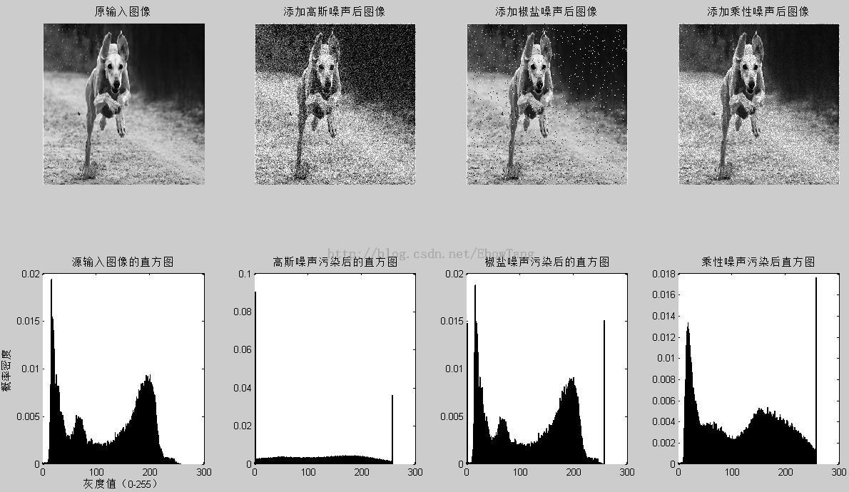
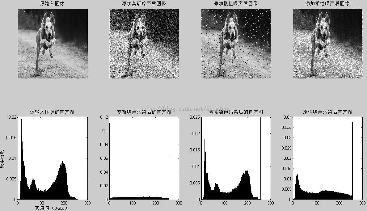
2，实验代码

<span style="font-size:12px;">%读入原始图像并显示
image_original=imread("dog.bmp");
figure(1)
subplot(2,4,1);
imshow(image_original);
title("原输入图像");
axis square;

%生成含高斯噪声图像并显示
pp=0.05;
image_gaosi_noise=imnoise(image_original,"gaussian",0,pp);
subplot(2,4,2);
imshow(image_gaosi_noise);
title("添加高斯噪声后图像");
axis square;

%生成含椒盐噪声图像并显示
d=0.05;
image_saltpepper_noise=imnoise(image_original,"salt & pepper",d);
subplot(2,4,3);
imshow(image_saltpepper_noise);
title("添加椒盐噪声后图像");
axis square;

%生成含乘性噪声图像并显示
var=0.05;
image_speckle_noise=imnoise(image_original,"speckle",var);
subplot(2,4,4);
imshow(image_speckle_noise);
title("添加乘性噪声后图像");
axis square;

%原图像直方图
r=0:255;  
bb=image_original(:); 
pg=hist(bb,r);  
pgr1=pg/length(bb);  
subplot(245);bar(pgr1);title("源输入图像的直方图");

r=0:255;  
bl=image_gaosi_noise(:); 
pg=hist(bl,r);  
pgr2=pg/length(bl);  
subplot(246);bar(pgr2);title("高斯噪声污染后的直方图");

r=0:255;  
bh=image_saltpepper_noise(:); 
pu=hist(bh,r);  
pgr3=pu/length(bh);  
subplot(247);bar(pgr3);title("椒盐噪声污染后的直方图");

r=0:255;  
ba=image_speckle_noise(:); 
pa=hist(ba,r);  
pgr4=pa/length(ba);  
subplot(248);bar(pgr4);title("乘性噪声污染后直方图");</span>

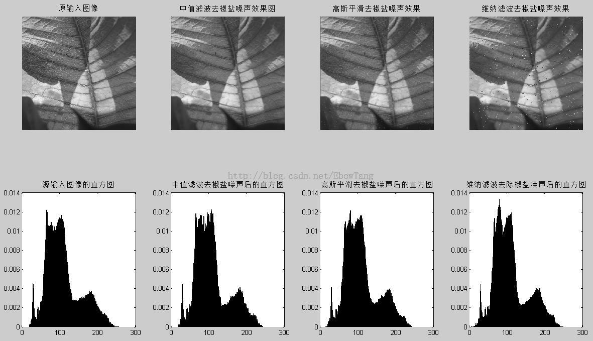
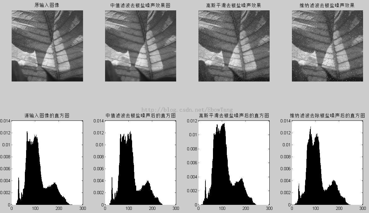
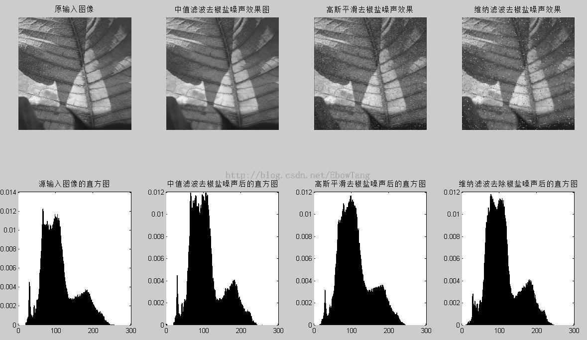
三，椒盐噪声去除能力对比

1，三大去噪效果

三幅图椒盐噪声浓度分别是0.01 0.03,0.05（比如第一副图均是加入0.01的椒盐噪声去噪对比）

2，实现代码

<span style="font-size:12px;"></span><pre name="code" class="cpp">%读入原始图像并显示
image_original=imread("dog.bmp");
figure(1)
subplot(2,4,1);
imshow(image_original);
title("原输入图像");
axis square;

%生成含高斯噪声图像并显示
%pp=0.05;
%image_gaosi_noise=imnoise(image_original,"gaussian",0,pp);

%生成含椒盐噪声图像并显示
dd=0.05;
image_saltpepper_noise=imnoise(image_original,"salt & pepper",dd);

%生成含乘性噪声图像并显示
%var=0.05;
%image_speckle_noise=imnoise(image_original,"speckle",var);

image_saltpepper_noise_after1=medfilt2(image_saltpepper_noise,[3,3]);
subplot(2,4,2);
imshow(image_saltpepper_noise_after1);title("中值滤波去椒盐噪声效果图");
axis square;

h_gaosi1=fspecial("gaussian",3,1);
image_saltpepper_noise_after2=imfilter(image_saltpepper_noise,h_gaosi1);
subplot(2,4,3);
imshow(image_saltpepper_noise_after2);title("高斯平滑去椒盐噪声效果");
axis square;

image_saltpepper_noise_after3=wiener2(image_saltpepper_noise,[5 5]);
subplot(2,4,4);
imshow(image_saltpepper_noise_after3);title("维纳滤波去椒盐噪声效果");
axis square;

%原图像直方图
r=0:255;  
bb=image_original(:); 
pg=hist(bb,r);  
pgr1=pg/length(bb);  
subplot(245);bar(pgr1);title("源输入图像的直方图");

r=0:255;  
bl=image_saltpepper_noise_after1(:); 
pg=hist(bl,r);  
pgr2=pg/length(bl);  
subplot(246);bar(pgr2);title("中值滤波去椒盐噪声后的直方图");

r=0:255;  
bh=image_saltpepper_noise_after2(:); 
pu=hist(bh,r);  
pgr3=pu/length(bh);  
subplot(247);bar(pgr3);title("高斯平滑去椒盐噪声后的直方图");

r=0:255;  
ba=image_saltpepper_noise_after3(:); 
pa=hist(ba,r);  
pgr4=pa/length(ba);  
subplot(248);bar(pgr4);title("维纳滤波去除椒盐噪声后的直方图");

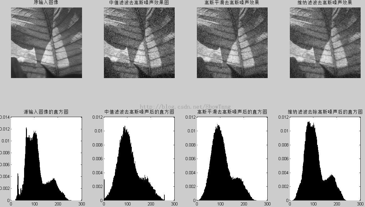
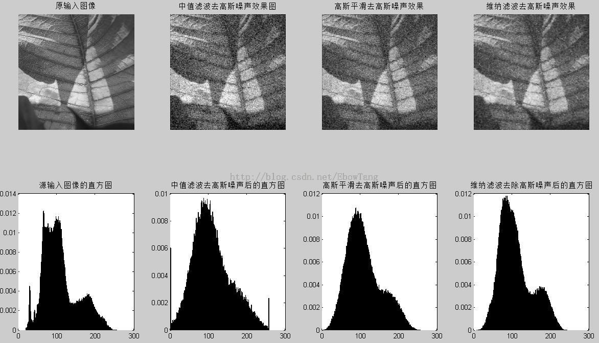
四，高斯噪声去除能力对比

1，去噪效果对比

2，实验代码

<span style="font-size:12px;"></span><pre name="code" class="cpp">%读入原始图像并显示
image_original=imread("dog.bmp");
figure(1)
subplot(2,4,1);
imshow(image_original);
title("原输入图像");
axis square;

%生成含高斯噪声图像并显示
pp=0.05;
image_gaosi_noise=imnoise(image_original,"gaussian",0,pp);

%生成含椒盐噪声图像并显示
%dd=0.01;
%image_saltpepper_noise=imnoise(image_original,"salt & pepper",dd);

%生成含乘性噪声图像并显示
%var=0.05;
%image_speckle_noise=imnoise(image_original,"speckle",var);

image_gaosi_noise_after1=medfilt2(image_gaosi_noise,[3,3]);
subplot(2,4,2);
imshow(image_gaosi_noise_after1);title("中值滤波去高斯噪声效果图");
axis square;

h_gaosi1=fspecial("gaussian",3,1);
image_gaosi_noise_after2=imfilter(image_gaosi_noise,h_gaosi1);
subplot(2,4,3);
imshow(image_gaosi_noise_after2);title("高斯平滑去高斯噪声效果");
axis square;

image_gaosi_noise_after3=wiener2(image_gaosi_noise,[5 5]);
subplot(2,4,4);
imshow(image_gaosi_noise_after3);title("维纳滤波去高斯噪声效果");
axis square;

%原图像直方图
r=0:255;  
bb=image_original(:); 
pg=hist(bb,r);  
pgr1=pg/length(bb);  
subplot(245);bar(pgr1);title("源输入图像的直方图");

r=0:255;  
bl=image_gaosi_noise_after1(:); 
pg=hist(bl,r);  
pgr2=pg/length(bl);  
subplot(246);bar(pgr2);title("中值滤波去高斯噪声后的直方图");

r=0:255;  
bh=image_gaosi_noise_after2(:); 
pu=hist(bh,r);  
pgr3=pu/length(bh);  
subplot(247);bar(pgr3);title("高斯平滑去高斯噪声后的直方图");

r=0:255;  
ba=image_gaosi_noise_after3(:); 
pa=hist(ba,r);  
pgr4=pa/length(ba);  
subplot(248);bar(pgr4);title("维纳滤波去除高斯噪声后的直方图");

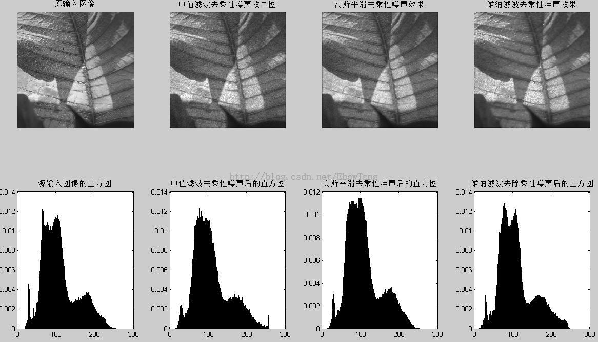
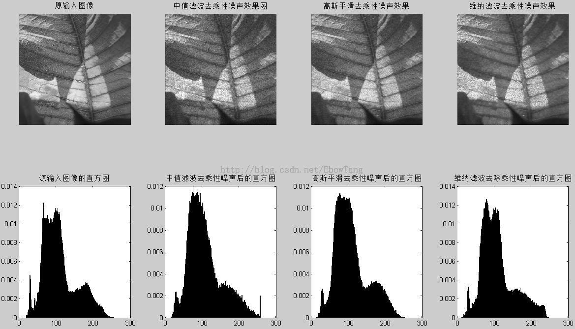
五，乘性噪声去除能力对比

1，去噪效果对比

2，实验代码

<span style="font-size:12px;">%读入原始图像并显示
image_original=imread("dog.bmp");
figure(1)
subplot(2,4,1);
imshow(image_original);
title("原输入图像");
axis square;

%生成含高斯噪声图像并显示
%pp=0.01;
%image_gaosi_noise=imnoise(image_original,"gaussian",0,pp);

%生成含椒盐噪声图像并显示
%dd=0.01;
%image_saltpepper_noise=imnoise(image_original,"salt & pepper",dd);

%生成含乘性噪声图像并显示
var=0.01;
image_speckle_noise=imnoise(image_original,"speckle",var);

image_speckle_noise_after1=medfilt2(image_speckle_noise,[3,3]);
subplot(2,4,2);
imshow(image_speckle_noise_after1);title("中值滤波去乘性噪声效果图");
axis square;

h_gaosi1=fspecial("gaussian",3,1);
image_speckle_noise_after2=imfilter(image_speckle_noise,h_gaosi1);
subplot(2,4,3);
imshow(image_speckle_noise_after2);title("高斯平滑去乘性噪声效果");
axis square;

image_speckle_noise_after3=wiener2(image_speckle_noise,[5 5]);
subplot(2,4,4);
imshow(image_speckle_noise_after3);title("维纳滤波去乘性噪声效果");
axis square;

%原图像直方图
r=0:255;  
bb=image_original(:); 
pg=hist(bb,r);  
pgr1=pg/length(bb);  
subplot(245);bar(pgr1);title("源输入图像的直方图");

r=0:255;  
bl=image_speckle_noise_after1(:); 
pg=hist(bl,r);  
pgr2=pg/length(bl);  
subplot(246);bar(pgr2);title("中值滤波去乘性噪声后的直方图");

r=0:255;  
bh=image_speckle_noise_after2(:); 
pu=hist(bh,r);  
pgr3=pu/length(bh);  
subplot(247);bar(pgr3);title("高斯平滑去乘性噪声后的直方图");

r=0:255;  
ba=image_speckle_noise_after3(:); 
pa=hist(ba,r);  
pgr4=pa/length(ba);  
subplot(248);bar(pgr4);title("维纳滤波去除乘性噪声后的直方图");</span>

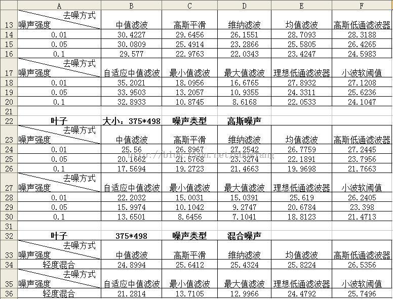
六，PNSR客观对比

（PNSR客观对比越高越好）

本对比也囊括了其他常见去噪方式的对比

参考资源

【1】《百度百科》

【2】《维基百科》

【3】冈萨雷斯《数字图像处理》

【4】http://blog.csdn.net/ebowtang/article/details/38960271