生成图表
如何分析用户的数据是一个有趣的问题,特别是当我们有大量的数据的时候。除了matlab,我们还可以用numpy+matplotlib
数据可以在这边寻找到
最后效果图
2014 01 01
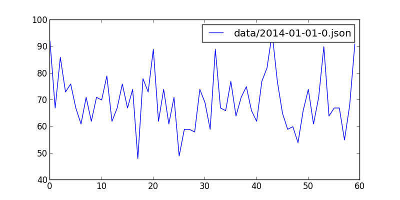
要解析的json文件位于data/2014-01-01-0.json,大小6.6M,显然我们可能需要用每次只读一行的策略,这足以解释为什么诸如sublime打开的时候很慢,而现在我们只需要里面的json数据中的创建时间。。
==,这个文件代表什么?
2014年1月1日零时到一时,用户在github上的操作,这里的用户指的是很多。。一共有4814条数据,从commit、create到issues都有。
数据解析
import json
for line in open(jsonfile):
    line = f.readline()
然后再解析json
import dateutil.parser

lin = json.loads(line)
date = dateutil.parser.parse(lin["created_at"])
这里用到了dateutil,因为新鲜出炉的数据是string需要转换为dateutil,再到数据放到数组里头。最后有就有了parse_data
def parse_data(jsonfile):
    f = open(jsonfile, "r")
    dataarray = []
    datacount = 0

    for line in open(jsonfile):
        line = f.readline()
        lin = json.loads(line)
        date = dateutil.parser.parse(lin["created_at"])
        datacount += 1
        dataarray.append(date.minute)

    minuteswithcount = [(x, dataarray.count(x)) for x in set(dataarray)]
    f.close()
    return minuteswithcount
下面这句代码就是将上面的解析为
minuteswithcount = [(x, dataarray.count(x)) for x in set(dataarray)]
这样的数组以便于解析
[(0, 92), (1, 67), (2, 86), (3, 73), (4, 76), (5, 67), (6, 61), (7, 71), (8, 62), (9, 71), (10, 70), (11, 79), (12, 62), (13, 67), (14, 76), (15, 67), (16, 74), (17, 48), (18, 78), (19, 73), (20, 89), (21, 62), (22, 74), (23, 61), (24, 71), (25, 49), (26, 59), (27, 59), (28, 58), (29, 74), (30, 69), (31, 59), (32, 89), (33, 67), (34, 66), (35, 77), (36, 64), (37, 71), (38, 75), (39, 66), (40, 62), (41, 77), (42, 82), (43, 95), (44, 77), (45, 65), (46, 59), (47, 60), (48, 54), (49, 66), (50, 74), (51, 61), (52, 71), (53, 90), (54, 64), (55, 67), (56, 67), (57, 55), (58, 68), (59, 91)]
Matplotlib
开始之前需要安装``matplotlib
sudo pip install matplotlib
然后引入这个库
import matplotlib.pyplot as plt
如上面的那个结果,只需要
    plt.figure(figsize=(8,4))
    plt.plot(x, y,label = files)
    plt.legend()
    plt.show()
最后代码可见
#!/usr/bin/env python
# -*- coding: utf-8 -*-

import json
import dateutil.parser
import numpy as np
import matplotlib.mlab as mlab
import matplotlib.pyplot as plt

def parse_data(jsonfile):
    f = open(jsonfile, "r")
    dataarray = []
    datacount = 0

    for line in open(jsonfile):
        line = f.readline()
        lin = json.loads(line)
        date = dateutil.parser.parse(lin["created_at"])
        datacount += 1
        dataarray.append(date.minute)

    minuteswithcount = [(x, dataarray.count(x)) for x in set(dataarray)]
    f.close()
    return minuteswithcount

def draw_date(files):
    x = []
    y = []
    mwcs = parse_data(files)
    for mwc in mwcs:
        x.append(mwc[0])
        y.append(mwc[1])

    plt.figure(figsize=(8,4))
    plt.plot(x, y,label = files)
    plt.legend()
    plt.show()

draw_date("data/2014-01-01-0.json")
每周分析
继上篇之后,我们就可以分析用户的每周提交情况,以得出用户的真正的工具效率,每个程序员的工作时间可能是不一样的,如
Phodal Huang’s Report
这是我的每周情况,显然如果把星期六移到前面的话,随着工作时间的增长,在github上的使用在下降,作为一个
a fulltime hacker who works best in the evening (around 8 pm).
不过这个是osrc的分析结果。
python github 每周情况分析
看一张分析后的结果
Feb Results
结果正好与我的情况相反?似乎图上是这么说的,但是数据上是这样的情况。
data
├── 2014-01-01-0.json
├── 2014-02-01-0.json
├── 2014-02-02-0.json
├── 2014-02-03-0.json
├── 2014-02-04-0.json
├── 2014-02-05-0.json
├── 2014-02-06-0.json
├── 2014-02-07-0.json
├── 2014-02-08-0.json
├── 2014-02-09-0.json
├── 2014-02-10-0.json
├── 2014-02-11-0.json
├── 2014-02-12-0.json
├── 2014-02-13-0.json
├── 2014-02-14-0.json
├── 2014-02-15-0.json
├── 2014-02-16-0.json
├── 2014-02-17-0.json
├── 2014-02-18-0.json
├── 2014-02-19-0.json
└── 2014-02-20-0.json
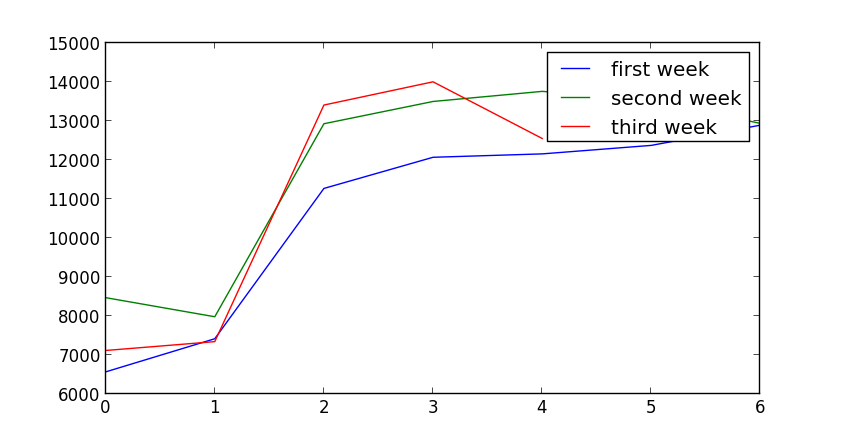
我们获取是每天晚上0点时的情况,至于为什么是0点,我想这里的数据量可能会比较少。除去1月1号的情况,就是上面的结果,在只有一周的情况时,总会以为因为在国内那时是假期,但是总觉得不是很靠谱,国内的程序员虽然很多,会在github上活跃的可能没有那么多,直至列出每一周的数据时。
  6570, 7420, 11274, 12073, 12160, 12378, 12897,
  8474, 7984, 12933, 13504, 13763, 13544, 12940,
  7119, 7346, 13412, 14008, 12555
Python 数据分析
重写了一个新的方法用于计算提交数,直至后面才意识到其实我们可以算行数就够了,但是方法上有点hack
def get_minutes_counts_with_id(jsonfile):
    datacount, dataarray = handle_json(jsonfile)
    minuteswithcount = [(x, dataarray.count(x)) for x in set(dataarray)]
    return minuteswithcount

def handle_json(jsonfile):
    f = open(jsonfile, "r")
    dataarray = []
    datacount = 0

    for line in open(jsonfile):
        line = f.readline()
        lin = json.loads(line)
        date = dateutil.parser.parse(lin["created_at"])
        datacount += 1
        dataarray.append(date.minute)

    f.close()
    return datacount, dataarray

def get_minutes_count_num(jsonfile):
    datacount, dataarray = handle_json(jsonfile)
    return datacount

def get_month_total():
    """

    :rtype : object
    """
    monthdaycount = []
    for i in range(1, 20):
        if i < 10:
            filename = "data/2014-02-0" + i.__str__() + "-0.json"
        else:
            filename = "data/2014-02-" + i.__str__() + "-0.json"
        monthdaycount.append(get_minutes_count_num(filename))
    return monthdaycount
接着我们需要去遍历每个结果,后面的后面会发现这个效率真的是太低了,为什么木有多线程?
Python Matplotlib图表
让我们的matplotlib来做这些图表的工作
if __name__ == "__main__":
    results = pd.get_month_total()
    print results

    plt.figure(figsize=(8, 4))
    plt.plot(results.__getslice__(0, 7), label="first week")
    plt.plot(results.__getslice__(7, 14), label="second week")
    plt.plot(results.__getslice__(14, 21), label="third week")
    plt.legend()
    plt.show()
蓝色的是第一周,绿色的是第二周,蓝色的是第三周就有了上面的结果。
我们还需要优化方法,以及多线程的支持。
让我们分析之前的程序,然后再想办法做出优化。网上看到一篇文章http://www.huyng.com/posts/python-performance-analysis/讲的就是分析这部分内容的。
存储到数据库中
SQLite3
我们创建了一个名为userdata.db的数据库文件,然后创建了一个表,里面有owner,language,eventtype,name url
def init_db():
    conn = sqlite3.connect("userdata.db")
    c = conn.cursor()
    c.execute("""CREATE TABLE userinfo (owner text, language text, eventtype text, name text, url text)""")
接着我们就可以查询数据,这里从结果讲起。
def get_count(username):
    count = 0
    userinfo = []
    condition = "select * from userinfo where owener = "" + str(username) + """
    for zero in c.execute(condition):
        count += 1
        userinfo.append(zero)

    return count, userinfo
当我查询gmszone的时候,也就是我自己就会有如下的结果
(u"gmszone", u"ForkEvent", u"RESUME", u"TeX", u"https://github.com/gmszone/RESUME")
(u"gmszone", u"WatchEvent", u"iot-dashboard", u"JavaScript", u"https://github.com/gmszone/iot-dashboard")
(u"gmszone", u"PushEvent", u"wechat-wordpress", u"Ruby", u"https://github.com/gmszone/wechat-wordpress")
(u"gmszone", u"WatchEvent", u"iot", u"JavaScript", u"https://github.com/gmszone/iot")
(u"gmszone", u"CreateEvent", u"iot-doc", u"None", u"https://github.com/gmszone/iot-doc")
(u"gmszone", u"CreateEvent", u"iot-doc", u"None", u"https://github.com/gmszone/iot-doc")
(u"gmszone", u"PushEvent", u"iot-doc", u"TeX", u"https://github.com/gmszone/iot-doc")
(u"gmszone", u"PushEvent", u"iot-doc", u"TeX", u"https://github.com/gmszone/iot-doc")
(u"gmszone", u"PushEvent", u"iot-doc", u"TeX", u"https://github.com/gmszone/iot-doc")
109
一共有109个事件,有Watch,Create,Push,Fork还有其他的, 项目主要有iot,RESUME,iot-dashboard,wechat-wordpress, 接着就是语言了,Tex,Javascript,Ruby,接着就是项目的url了。
值得注意的是。
-rw-r--r-- 1 fdhuang staff 905M Apr 12 14:59 userdata.db
这个数据库文件有905M,不过查询结果相当让人满意,至少相对于原来的结果来说。
Python自带了对SQLite3的支持,然而我们还需要安装SQLite3
brew install sqlite3
或者是
sudo port install sqlite3
或者是Ubuntu的
sudo apt-get install sqlite3
openSUSE自然就是
sudo zypper install sqlite3
不过,用yast2也很不错,不是么。。
数据导入
需要注意的是这里是需要python2.7,起源于对gzip的上下文管理器的支持问题
def handle_gzip_file(filename):
    userinfo = []
    with gzip.GzipFile(filename) as f:
        events = [line.decode("utf-8", errors="ignore") for line in f]

        for n, line in enumerate(events):
            try:
                event = json.loads(line)
            except:

                continue

            actor = event["actor"]
            attrs = event.get("actor_attributes", {})
            if actor is None or attrs.get("type") != "User":
                continue

            key = actor.lower()

            repo = event.get("repository", {})
            info = str(repo.get("owner")), str(repo.get("language")), str(event["type"]), str(repo.get("name")), str(
                repo.get("url"))
            userinfo.append(info)

    return userinfo

def build_db_with_gzip():
    init_db()
    conn = sqlite3.connect("userdata.db")
    c = conn.cursor()

    year = 2014
    month = 3

    for day in range(1,31):
        date_re = re.compile(r"([0-9]{4})-([0-9]{2})-([0-9]{2})-([0-9]+).json.gz")

        fn_template = os.path.join("march",
                                   "{year}-{month:02d}-{day:02d}-{n}.json.gz")
        kwargs = {"year": year, "month": month, "day": day, "n": "*"}
        filenames = glob.glob(fn_template.format(**kwargs))

        for filename in filenames:
            c.executemany("INSERT INTO userinfo VALUES (?,?,?,?,?)", handle_gzip_file(filename))

    conn.commit()
    c.close()
executemany可以插入多条数据,对于我们的数据来说,一小时的文件大概有五六千个会符合我们上面的安装,也就是有actor又有type才是我们需要记录的数据,我们只需要统计用户的那些事件,而非全部的事件。
我们需要去遍历文件,然后找到合适的部分,这里只是要找2014-03-01到2014-03-31的全部事件,而光这些数据的gz文件就有1.26G,同上面那些解压为json文件显得不合适,只能用遍历来处理。
这里参考了osrc项目中的写法,或者说直接复制过来。
首先是正规匹配
date_re = re.compile(r"([0-9]{4})-([0-9]{2})-([0-9]{2})-([0-9]+).json.gz")
不过主要的还是在于glob.glob
glob是python自己带的一个文件操作相关模块,用它可以查找符合自己目的的文件,就类似于Windows下的文件搜索,支持通配符操作。
这里也就用上了gzip.GzipFile又一个不错的东西。
最后代码可以见
更好的方案?
Redis
查询用户事件总数
import redis
r = redis.StrictRedis(host="localhost", port=6379, db=0)
pipe = pipe = r.pipeline()
pipe.zscore("osrc:user","gmszone")
pipe.execute()
系统返回了227.0,试试别人。
>>> pipe.zscore("osrc:user","dfm")
<redis.client.StrictPipeline object at 0x104fa7f50>
>>> pipe.execute()
[425.0]
>>>
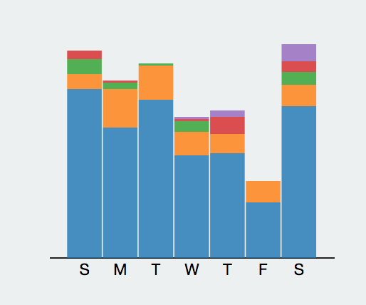
看看主要是在哪一天提交的
>>> pipe.hgetall("osrc:user:gmszone:day")
<redis.client.StrictPipeline object at 0x104fa7f50>
>>> pipe.execute()
[{"1": "51", "0": "41", "3": "17", "2": "34", "5": "28", "4": "22", "6": "34"}]
结果大致如下图所示:
SMTWTFS
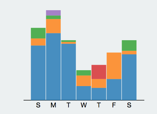
看看主要的事件是?
>>> pipe.zrevrange("osrc:user:gmszone:event".format("gmszone"), 0, -1,withscores=True)
<redis.client.StrictPipeline object at 0x104fa7f50>
>>> pipe.execute()
[[("PushEvent", 154.0), ("CreateEvent", 41.0), ("WatchEvent", 18.0), ("GollumEvent", 8.0), ("MemberEvent", 3.0), ("ForkEvent", 2.0), ("ReleaseEvent", 1.0)]]
>>>
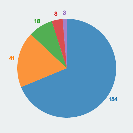
Main Event
蓝色的就是push事件,黄色的是create等等。
到这里我们算是知道了OSRC的数据库部分是如何工作的。
Redis 查询
主要代码如下所示
def get_vector(user, pipe=None):

    r = redis.StrictRedis(host="localhost", port=6379, db=0)
    no_pipe = False
    if pipe is None:
        pipe = pipe = r.pipeline()
        no_pipe = True

    user = user.lower()
    pipe.zscore(get_format("user"), user)
    pipe.hgetall(get_format("user:{0}:day".format(user)))
    pipe.zrevrange(get_format("user:{0}:event".format(user)), 0, -1,
                   withscores=True)
    pipe.zcard(get_format("user:{0}:contribution".format(user)))
    pipe.zcard(get_format("user:{0}:connection".format(user)))
    pipe.zcard(get_format("user:{0}:repo".format(user)))
    pipe.zcard(get_format("user:{0}:lang".format(user)))
    pipe.zrevrange(get_format("user:{0}:lang".format(user)), 0, -1,
                   withscores=True)

    if no_pipe:
        return pipe.execute()
结果在上一篇中显示出来了,也就是
[227.0, {"1": "51", "0": "41", "3": "17", "2": "34", "5": "28", "4": "22", "6": "34"}, [("PushEvent", 154.0), ("CreateEvent", 41.0), ("WatchEvent", 18.0), ("GollumEvent", 8.0), ("MemberEvent", 3.0), ("ForkEvent", 2.0), ("ReleaseEvent", 1.0)], 0, 0, 0, 11, [("CSS", 74.0), ("JavaScript", 60.0), ("Ruby", 12.0), ("TeX", 6.0), ("Python", 6.0), ("Java", 5.0), ("C++", 5.0), ("Assembly", 5.0), ("C", 3.0), ("Emacs Lisp", 2.0), ("Arduino", 2.0)]]
有意思的是在这里生成了和自己相近的人
["alesdokshanin", "hjiawei", "andrewreedy", "christj6", "1995eaton"]
osrc最有意思的一部分莫过于flann,当然说的也是系统后台的设计的一个很关键及有意思的部分。
邻近算法与相似用户
邻近算法是在这个分析过程中一个很有意思的东西。
邻近算法,或者说K最近邻(kNN,k-NearestNeighbor)分类算法可以说是整个数据挖掘分类技术中最简单的方法了。所谓K最近邻,就是k个最近的邻居的意思,说的是每个样本都可以用她最接近的k个邻居来代表。
换句话说,我们需要一些样本来当作我们的分析资料,这里东西用到的就是我们之前的。
[227.0, {"1": "51", "0": "41", "3": "17", "2": "34", "5": "28", "4": "22", "6": "34"}, [("PushEvent", 154.0), ("CreateEvent", 41.0), ("WatchEvent", 18.0), ("GollumEvent", 8.0), ("MemberEvent", 3.0), ("ForkEvent", 2.0), ("ReleaseEvent", 1.0)], 0, 0, 0, 11, [("CSS", 74.0), ("JavaScript", 60.0), ("Ruby", 12.0), ("TeX", 6.0), ("Python", 6.0), ("Java", 5.0), ("C++", 5.0), ("Assembly", 5.0), ("C", 3.0), ("Emacs Lisp", 2.0), ("Arduino", 2.0)]]
在代码中是构建了一个points.h5的文件来分析每个用户的points,之后再记录到hdf5文件中。
[ 0.00438596  0.18061674  0.2246696   0.14977974  0.07488987  0.0969163
    0.12334802  0.14977974  0.          0.18061674  0.          0.          0.
    0.00881057  0.          0.          0.03524229  0.          0.
    0.01321586  0.          0.          0.          0.6784141   0.
    0.07929515  0.00440529  1.          1.          1.          0.08333333
    0.26431718  0.02202643  0.05286344  0.02643172  0.          0.01321586
    0.02202643  0.          0.          0.          0.          0.          0.
    0.          0.          0.00881057  0.          0.          0.          0.
    0.          0.          0.          0.          0.          0.          0.
    0.          0.          0.          0.          0.00881057]
这里分析到用户的大部分行为,再找到与其行为相近的用户,主要的行为有下面这些:
- 每星期的情况
- 事件的类型
- 贡献的数量,连接以及语言
- 最多的语言
osrc中用于解析的代码
def parse_vector(results):
    points = np.zeros(nvector)
    total = int(results[0])

    points[0] = 1.0 / (total + 1)

    # Week means.
    for k, v in results[1].iteritems():
        points[1 + int(k)] = float(v) / total

    # Event types.
    n = 8
    for k, v in results[2]:
        points[n + evttypes.index(k)] = float(v) / total

    # Number of contributions, connections and languages.
    n += nevts
    points[n] = 1.0 / (float(results[3]) + 1)
    points[n + 1] = 1.0 / (float(results[4]) + 1)
    points[n + 2] = 1.0 / (float(results[5]) + 1)
    points[n + 3] = 1.0 / (float(results[6]) + 1)

    # Top languages.
    n += 4
    for k, v in results[7]:
        if k in langs:
            points[n + langs.index(k)] = float(v) / total
        else:
            # Unknown language.
            points[-1] = float(v) / total

    return points
这样也就返回我们需要的点数,然后我们可以用get_points来获取这些
def get_points(usernames):
    r = redis.StrictRedis(host="localhost", port=6379, db=0)
    pipe = r.pipeline()

    results = get_vector(usernames)
    points = np.zeros([len(usernames), nvector])
    points = parse_vector(results)
    return points
就会得到我们的相应的数据,接着找找和自己邻近的,看看结果。
[ 0.01298701  0.19736842  0.          0.30263158  0.21052632  0.19736842
    0.          0.09210526  0.          0.22368421  0.01315789  0.          0.
    0.          0.          0.          0.01315789  0.          0.
    0.01315789  0.          0.          0.          0.73684211  0.          0.
    0.          1.          1.          1.          0.2         0.42105263
    0.09210526  0.          0.          0.          0.          0.23684211
    0.          0.          0.03947368  0.          0.          0.          0.
    0.          0.          0.          0.          0.          0.          0.
    0.          0.          0.          0.          0.          0.          0.
    0.          0.          0.          0.        ]
真看不出来两者有什么相似的地方 。。。。